Introduction

전이학습이라는 어느 한 문제에서 학습된 feature를 가지고 비슷하면서 새로운 문제에 이를 활용하는 방법이다 예를들어 너구리를 식별하는 모델로 부터의 features는 tanuki(대충 너구리 비슷한놈)을 구별하는데 유용하다 또한 전이학습은 내가 가지고있는데 큰 규모의 모델을 학습하는데 있어 dataset이 매우 적을때 유용하다.

전이학습의 일반적인 활용은 아래와 같다.

1. 미리 학습된 모델로부터의 layer을 가져온다.

2. 그것들이 가지고 있는 어느 정보가 layer가 앞으로 학습되는데 있어 총둘을 야기시키기 떄문에 Freeze해준다

3. frozen된 layer위에 trainable layers를 더해준다 그것들은 이전의 학습된 특징으로부터 새로운 dataset에 의한 예측값으로 변할 것이다.

4. new layers를 내가 가지고있는 dataset으로 학습시킨다.

마지막으로 선택적인 단계가 있는데 fine-tuning이다 이는 위에서 획득한 전체 모델을 고정해제하는 것으로 구성된다 그리고 다시 새로운 데이터로 매우 느린 학습률을 가진채로 재학습시킨다. 이는 잠재적으로 의미있는 향상을 보인다 또한 사전 훈련 된 기능을 새 데이터에 점진적으로 적용는 것이다.

우선 Keras trainable API을 자세히 살펴볼 것이다 이는 대부분의 전이학습과 fine-tunung작업의 기초라 할 수 있다. 그리고 특정한 workflow를 증명할 것이다 ImageNet에 미리 학습된 모델을 가져옴으로써 그리고 “cats vs dogs 구별 데이터셋을 재학습 시킴으로써

freezing layers: understanding the trainable attribute

Layers & models은 가중치요소를 가지고있다.

• weight는 layer에 있는 모든 가중치의 리스트이다

• trainable_weights는 학습동안 loss함수의 최소화에 있어 계속되어 업데이트되는 가중치 리스트이다

• non_trainable_weight는 학습되지 않는 것들을 의미한다 특히 forward pass동안 모델에 의해 업데이트 된다.

아래 예시를 보자

layer = keras.layers.Dense(3)
layer.build((None, 4))  # Create the weights

print("weights:", len(layer.weights))
print("trainable_weights:", len(layer.trainable_weights))
print("non_trainable_weights:", len(layer.non_trainable_weights))


결과
weights: 2
trainable_weights: 2
non_trainable_weights: 0

일반적으로 모든 가중치들은 훈련가능한 가중치이다 학습하지 않는 layer는 BatchNormarlization층 밖에 없다 학습하는 동안 input의 mean과 variance를 추적할때 non-trainalble을 사용한다 .

Example: the BatchNormalization layer has 2 trainable weights and 2 non-trainable weights

layer = keras.layers.BatchNormalization()
layer.build((None, 4))  # Create the weights

print("weights:", len(layer.weights))
print("trainable_weights:", len(layer.trainable_weights))
print("non_trainable_weights:", len(layer.non_trainable_weights))\

결과
weights: 4
trainable_weights: 2
non_trainable_weights: 2

Layers & model은 trainable에 있어 이중적인 특징을 가진다 이것의 값은 바꿀 수 있다 layer.trainable을 False로 세팅하는 것은 layer에 weights들을 trainable 에서 non-tranable 하게 만든다. 이를 두고 “freezing”이라 부른다. 이렇게 frozen되어있는 layer는 학습하는 동안 업데이트 되지 않는다.

EXAMPLE: setting trainable to False

layer = keras.layers.Dense(3)
layer.build((None, 4))  # Create the weights
layer.trainable = False  # Freeze the layer

print("weights:", len(layer.weights))
print("trainable_weights:", len(layer.trainable_weights))
print("non_trainable_weights:", len(layer.non_trainable_weights))

결과
weights: 2
trainable_weights: 0
non_trainable_weights: 2
# trainable_weight이 2개가 사라짐

trainable weight가 non-trainable하게 될때 그 값은 더이상 학습하는 동안 업데이트 되지 않는다.

# Make a model with 2 layers
layer1 = keras.layers.Dense(3, activation="relu")
layer2 = keras.layers.Dense(3, activation="sigmoid")
model = keras.Sequential([keras.Input(shape=(3,)), layer1, layer2])

# Freeze the first layer
layer1.trainable = False

# Keep a copy of the weights of layer1 for later reference
initial_layer1_weights_values = layer1.get_weights()

# Train the model
model.compile(optimizer="adam", loss="mse")
model.fit(np.random.random((2, 3)), np.random.random((2, 3)))

# Check that the weights of layer1 have not changed during training
final_layer1_weights_values = layer1.get_weights()
np.testing.assert_allclose(
    initial_layer1_weights_values[0], final_layer1_weights_values[0]
)
np.testing.assert_allclose(
    initial_layer1_weights_values[1], final_layer1_weights_values[1]
)

recursive setting of the trainable attribute

만약 sublayer를 가지거나 children layer가 있는 layer를 trainable =false로 설정헀다면 이는 하위의 layer들도 non-trainable해진다 example

inner_model = keras.Sequential(
    [
        keras.Input(shape=(3,)),
        keras.layers.Dense(3, activation="relu"),
        keras.layers.Dense(3, activation="relu"),
    ]
)

model = keras.Sequential(
    [keras.Input(shape=(3,)), inner_model, keras.layers.Dense(3, activation="sigmoid"),]
)

model.trainable = False  # Freeze the outer model

assert inner_model.trainable == False  # All layers in `model` are now frozen
assert inner_model.layers[0].trainable == False  # `trainable` is propagated recursively

Typical transfer-learning workflow

Keras에서 특정한 전이학습과정이 어떻게 이루어지는지를 알아보자

1. 기반 모델을 인스턴트화하고 학습된 weight를 로드하여 모델에 넣는다

2. 기반 모델에 있는 모든 layers를 고정한다 (trainable = False를 통해)

3. 기반 모델의 output layer위에 새로운 모델을 생성한다.

4. 새로운 데이터로 새로운 모델을 학습하자!

더욱 가벼운 작업에 있어 또한 이러한 대안이 있다.

1. 기반 모델을 인스턴트화하고 학습된 weight를 로드하여 모델에 넣는다.

2. 새로운 데이터를 이용해 원래 모델을 통해 학습시킨다 그리고 결과물중 하나의 layer를 저장한다 이를 feature extraction(특징 추출)이라고 부른다

3. 이렇게 나온 출력값을 비슷한(가벼운)모델에 input 데이터로 사용한다.

아래에서는 첫번째 workflow를 따라 보겠다.

1. 먼저 사전 훈련된 가중치로 기본모델을 .instance화 한다

   base_model = keras.applications.Xception(
    weights='imagenet',  # Load weights pre-trained on ImageNet.
    input_shape=(150, 150, 3),
    include_top=False)  # Do not include the ImageNet classifier at the top.
   

여기서 Xceptiom이라는 모델이 나오는데 이에대하여 알아보자

Xception

Pretrained된 모델을 사용하거나 transfer Learning을 사용하는 모델들에 대해서 읽을 떄 가장 근본이되는 CNN모델들이 몇개 있다 ex)VSG family , ResNet family , Inception family 마지막으로 Xception

Xception모델이란 구글이 2017년에 발표한 모델로 Encoder-Decoder 형태의 모델들에서 pretrain된 Xception모델이 Encoder로 자주 쓰인다 또한 Xception에서 제시하는 모델의 구조나 핵심인 modified depthwise separable convolution의 개념이 간단하기 때문에 다른 모델에도 적용하기 쉽다. Xception 이라는 이름자체가 Extreame + Inception에서 나온 만큼 Inception모델이 기본이 된다는 것이다 따라서 iNCEPTION에 대해 간단히 알아보자

Inception Family

Inception 모델은 지금까지 version 4과 ResNet이 합쳐진 Inception-ResNet v2 까지 나왔습니다. 딥러닝은 망이 깊을수록, 레이어가 넓을 수록 성능이 좋지만 overfitting문제로 깊고 넓게만 모델을 만드는건 문제가 된다. Inception은 Convolution 레이어를 부족(sparse)하게 연결하면서 행렬연산은 dense하게 처리하기 위해 고안한 모델이다.

다른 Convolution과 다른점이란 보통 5x5 또는 7X7의 하나의 CONVOLUTION 필터로 진행하는데 inception모델로 진행하는데 Inception 모델에서는 conv 레이어 여러 개를 한 층에서 구성하는 형태를 취하고 있습니다.

왜이렇게 하는가? 이는 Parameter의 갯수도 줄이고 연산량도 줄일수 있기 떄문이다 이떄 위 그림과 다르게 Kenel size가 늘어날수록 연산량의 크기가 굉장히 커지기 떄문에 5x5가 아니라 3x3을 두번하는 방향으로 바뀐다 - 이또한 더욱 쪼개질 수 있다.

-1x1 Conv를 하는 이유는 보통의 convolution이 채널의 개수를 늘리지만 1x1연산의 목적은 채널의 개수를 줄여서 압축하는데에 있다. 이를 Residual Network라고 하는데

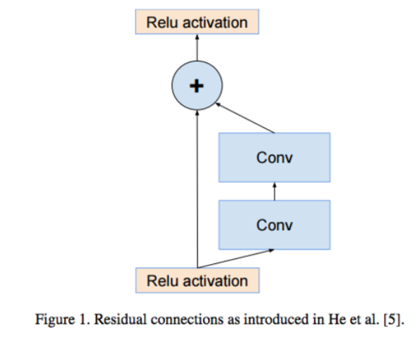
학습수렴속도가 빨라진다는 장점이 있다

즉 정리하자면 Inception 모델들의 내용은 Convolution 을 할 때 하나의 큰 kernel 을 사용할게 아니라 다양한 크기를 이어붙이는것이 연산량 & parameter의 개수도 적도, 좋은 결과를 얻을 수 있다 거기에 ResNet 넣으면 수렴속도도 빨라진다.

자 그럼 Xception에 대해 알아보자 Xception의 중점포인트: Modified Depthwise Separable Convolution Xception의 목적은 연산량과 parameter의 개수를 줄여서, 큰 이미지 인식을 고속화 시키는 것이다.

장점: VSG처럼 네트워크의 구조가 간단해서 위의 inception과 달리 활용도가 높다.

Xception의 바탕이 된 개념들을 살펴보도록하면 1. VGG16의 구조- deep하게 쌓아가는 구조를 따온 점 2. inception Family: Conv를 할 때 몇개의 branch로 factorize 해서 진행하는 것의 장점을 알려준점 3. Depthwise Separable Convolution 네트워크의 사이즈와 연산량을 줄이기 위한 연구 (채널별로 conv를 진행한 후 space에 대해서 conv를 진행한다)

Modified Depthwise Separable Convolution

원래의 Modified Depthwise Separable Convolution는 무엇인가?

-Depthwise(깊이 별로 == 채널 별로) Separable(나누어서) convolution 을 하는 것! 일반 Convolution과 결과는 같지만 두 단계로 진행된다

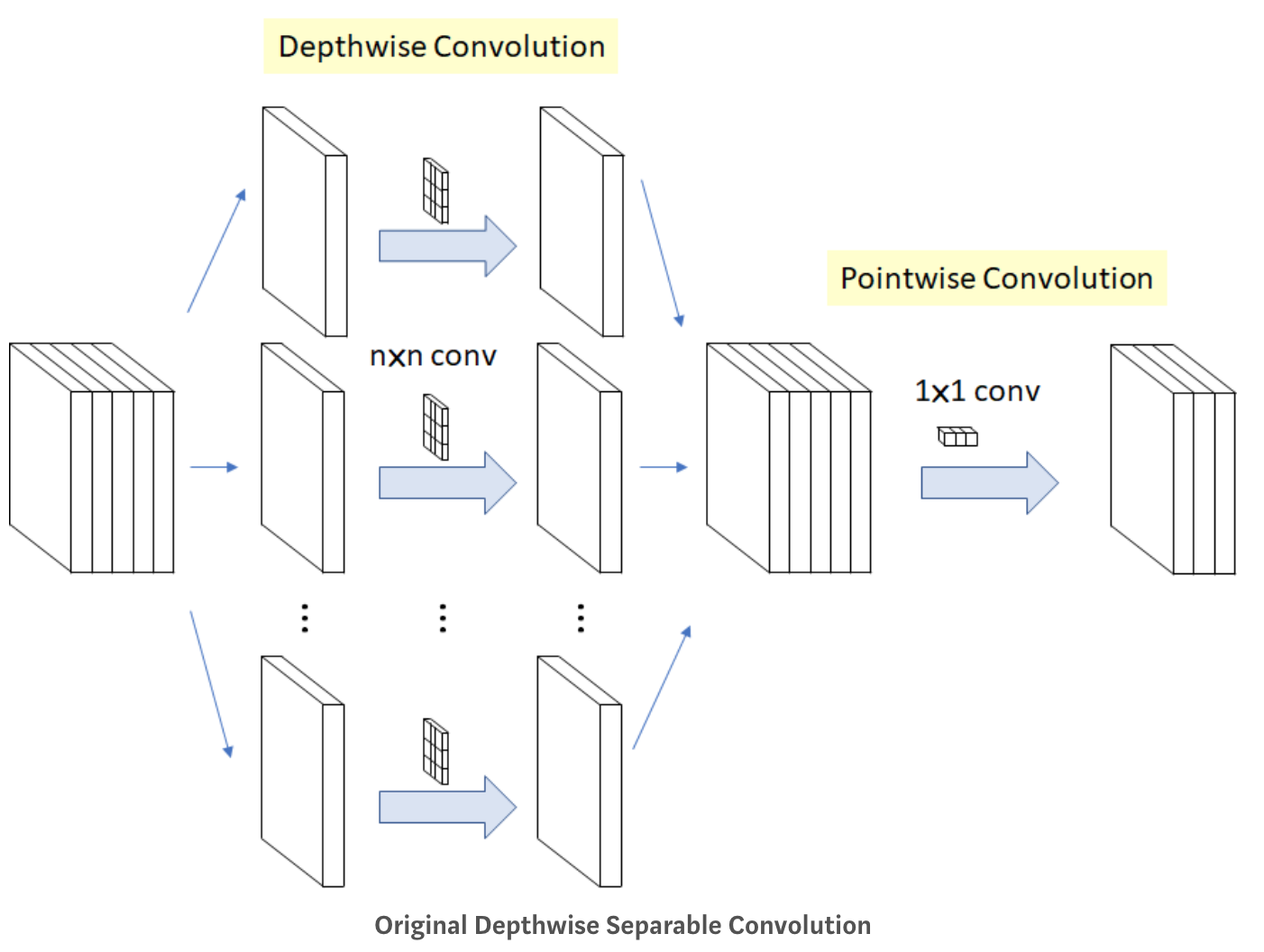
1단계: Channel-wise nxn spatial convolution: 위에 그림에서와 같이 인풋으로 5개의 채널이 들어오면 5개의 n x n convolution 을 따로 진행해서 합칩니다.

2단계: Pointwise Convolution: 원래 우리가 알고있는 1x1 convolution입니다. 채널의 개수를 줄이기 위한 방법으로 사용됩니다.

요는 이렇게 사용한다

def xception(pretrained=False,**kwargs):

    model = Xception(**kwargs)
    if pretrained:
        model.load_state_dict(model_zoo.load_url(model_urls['xception']))
    return model

자 다시 전이 학습으로 돌아가자 모델을 인스턴스화 한뒤 기본 모델을 고정한다

base_model.trainable = False

위에 새모델을 만든다 `` inputs = keras.Input(shape=(150, 150, 3))

We make sure that the base_model is running in inference mode here,

by passing training=False. This is important for fine-tuning, as you will

learn in a few paragraphs.

x = base_model(inputs, training=False)

Convert features of shape base_model.output_shape[1:] to vectors

x = keras.layers.GlobalAveragePooling2D()(x)

A Dense classifier with a single unit (binary classification)

outputs = keras.layers.Dense(1)(x) model = keras.Model(inputs, outputs) `` 훈련시킨다

model.compile(optimizer=keras.optimizers.Adam(),
              loss=keras.losses.BinaryCrossentropy(from_logits=True),
              metrics=[keras.metrics.BinaryAccuracy()])
model.fit(new_dataset, epochs=20, callbacks=..., validation_data=...)

fine-tuning (미세 조정)

모델이 새 데이터에 수렴되면 기본 모델의 전체 또는 일부를 고정 해제하고 매우 낮은 학습률로 전체 모델을 종단 간 다시 훈련 할 수 있습니다.

이는 잠재적으로 점진적 개선을 제공 할 수있는 선택적 마지막 단계입니다. 또한 잠재적으로 빠른 과적 합으로 이어질 수 있습니다.

고정 된 레이어가있는 모델이 수렴하도록 훈련 된 후에 만이 단계를 수행하는 것이 중요합니다. 무작위로 초기화 된 학습 가능 레이어를 사전 학습 된 기능을 보유하는 학습 가능한 레이어와 혼합하면 무작위로 초기화 된 레이어로 인해 학습 중에 매우 큰 그라데이션 업데이트가 발생하여 사전 학습 된 기능이 파괴됩니다.

일반적으로 매우 작은 데이터 세트에서 첫 번째 학습 단계보다 훨씬 더 큰 모델을 학습하기 때문에이 단계에서 매우 낮은 학습률을 사용하는 것도 중요합니다. 결과적으로 큰 체중 업데이트를 적용하면 매우 빠르게 과적 합할 위험이 있습니다. 여기서는 사전 훈련 된 가중치를 증분 방식으로 만 재조정하려고합니다.

다음은 전체 기본 모델의 미세 조정을 구현하는 방법입니다.

# Unfreeze the base model
base_model.trainable = True

# It's important to recompile your model after you make any changes
# to the `trainable` attribute of any inner layer, so that your changes
# are take into account
model.compile(optimizer=keras.optimizers.Adam(1e-5),  # Very low learning rate
              loss=keras.losses.BinaryCrossentropy(from_logits=True),
              metrics=[keras.metrics.BinaryAccuracy()])

# Train end-to-end. Be careful to stop before you overfit!
model.fit(new_dataset, epochs=10, callbacks=..., validation_data=...)

BatchNormalization 계층에 대한 중요 참고사항

많은 이미지 모델에는 BatchNormalization 레이어가 포함되어 있습니다. 그 레이어는 모든 상상할 수있는 특별한 경우입니다. 명심해야 할 몇 가지 사항이 있습니다. BatchNormaliztion에는 훈련중에 업데이트되는 2개의 non-trainable weight가 포함된다 입력값의 평균과 분산을 추적하는 변수이다.

bn_layer.trainable = False를 설정하면 BatchNormalization계층이 추론모드에서 실행되고 평균 및 분산 통계를 업데이트 하지 않습니다

미세조정을 수행하기 위해 BatchNormalization레이어가 포함된 모델을 BatchNormalization하는 경우 기본 모델을 호출할 때 trainaing= False를 전달하여 BatchNormalization레이어를 추론모드로 유지해야한다 그렇지 않으면 훈련 부가능한 가중치에 적용된 업데이트가 모델이 학습한 내용을 갑자기 파괴한다.

end to end 예제 : 고양이와 개에 대한 이미지 분류모델 미세조정

데이터세트:

이러한 개념을 구체화하기 위해 구체적인 종단 간 전이 학습 및 미세 조정 예제를 살펴 보겠습니다. ImageNet에서 사전 훈련 된 Xception 모델을로드하고 Kaggle “cats vs. dogs”분류 데이터 셋에서 사용합니다.

데이터 얻기:

먼저 TFDS를 사용하여 cats vs dogs dataset을 가져온다 전이학습은 매우 작은 dataset로 작업할 때 가장 유용하다 데이터 세트를 작게 유지하기 위해 원래 훈련데이터 (25000)개의 이미지의 40%를 훈련에 10&를 검증에 10%를 테스트에 사용한다 .

import tensorflow_datasets as tfds

tfds.disable_progress_bar()

train_ds, validation_ds, test_ds = tfds.load(
    "cats_vs_dogs",
    # Reserve 10% for validation and 10% for test
    split=["train[:40%]", "train[40%:50%]", "train[50%:60%]"],
    as_supervised=True,  # Include labels
)

print("Number of training samples: %d" % tf.data.experimental.cardinality(train_ds))
print(
    "Number of validation samples: %d" % tf.data.experimental.cardinality(validation_ds)
)
print("Number of test samples: %d" % tf.data.experimental.cardinality(test_ds))

정말 유용한것 같다 특히 “split=[“train[:40%]”, “train[40%:50%]”, “train[50%:60%]”],” 이부분 이런식으로 데이터를 나눌 수 있다.

import matplotlib.pyplot as plt

plt.figure(figsize=(10, 10))
for i, (image, label) in enumerate(train_ds.take(9)):
    ax = plt.subplot(3, 3, i + 1)
    plt.imshow(image)
    plt.title(int(label))
    plt.axis("off")

label 1이 ‘dog’ 이고 label 2가 ‘cat’이다

데이터 표준화

원시 이미지의 크기는 다양합니다. 또한 각 픽셀은 0에서 255 사이의 3 개의 정수 값 (RGB 수준 값)으로 구성됩니다. 이것은 신경망을 공급하는 데 적합하지 않습니다. 다음 두 가지를 수행해야합니다.

• 고정된 이미지 크기로 표준화한다 150x150을 선택한다

• -1과 1 사이의 픽셀 값을 Normalization 합니다. 모델 자체의 일부로 Normalization 레이어를 사용하여이 작업을 수행합니다.

일반적으로 이미 사전 처리 된 데이터를 사용하는 모델과 달리 원시 데이터를 입력으로 사용하는 모델을 개발하는 것이 좋습니다. 그 이유는 모델이 사전 처리 된 데이터를 예상하는 경우 모델을 내보내 다른 곳 (웹 브라우저, 모바일 앱)에서 사용할 때마다 정확히 동일한 사전 처리 파이프 라인을 다시 구현해야하기 때문입니다. 이것은 매우 빠르게 매우 까다로워집니다. 따라서 모델에 도달하기 전에 가능한 최소한의 전처리 작업을 수행해야합니다.

여기서는 데이터 파이프 라인에서 이미지 크기 조정을 수행하고 (심층 신경망은 연속 된 데이터 배치 만 처리 할 수 ​​있기 때문에) 모델을 생성 할 때 입력 값 크기 조정을 모델의 일부로 수행합니다.

size = (150, 150)

train_ds = train_ds.map(lambda x, y: (tf.image.resize(x, size), y))
validation_ds = validation_ds.map(lambda x, y: (tf.image.resize(x, size), y))
test_ds = test_ds.map(lambda x, y: (tf.image.resize(x, size), y))

밑은 데이터를 일괄처리하고 cashing 및 free patch를 사용하여 로딩 속도를 최적화 한것이다

batch_size = 32

train_ds = train_ds.cache().batch(batch_size).prefetch(buffer_size=10)
validation_ds = validation_ds.cache().batch(batch_size).prefetch(buffer_size=10)
test_ds = test_ds.cache().batch(batch_size).prefetch(buffer_size=10)

무작위 data증가 사용

큰 이미지 데이터 세트가없는 경우 무작위 수평 뒤집기 또는 작은 무작위 회전과 같은 무작위이지만 사실적인 변환을 훈련 이미지에 적용하여 샘플 다양성을 인위적으로 도입하는 것이 좋습니다. 이를 통해 과적 합 속도를 늦추면서 학습 데이터의 다양한 측면에 모델을 노출 할 수 있습니다.

from tensorflow import keras
from tensorflow.keras import layers

data_augmentation = keras.Sequential(
    [
        layers.experimental.preprocessing.RandomFlip("horizontal"),
        layers.experimental.preprocessing.RandomRotation(0.1),
    ]
)

import numpy as np

for images, labels in train_ds.take(1):
    plt.figure(figsize=(10, 10))
    first_image = images[0]
    for i in range(9):
        ax = plt.subplot(3, 3, i + 1)
        augmented_image = data_augmentation(
            tf.expand_dims(first_image, 0), training=True
        )
        plt.imshow(augmented_image[0].numpy().astype("int32"))
        plt.title(int(labels[i]))
        plt.axis("off")

변환된 이미지를 살펴보도록하자

#### 모델구축

참고:

• Normalization 레이어를 추가하여 입력 값 (처음에는 [0, 255] 범위)을 [-1, 1] 범위로 조정합니다.

• 정규화를 위해 분류 계층 앞에 Dropout 계층을 추가합니다.

• 기본 모델을 호출 할 때 training=False 를 전달하여 추론 모드에서 실행되도록하여 미세 조정을 위해 기본 모델을 고정 해제 한 후에도 batchnorm 통계가 업데이트되지 않도록합니다.

 base_model = keras.applications.Xception(
    weights="imagenet",  # Load weights pre-trained on ImageNet.
    input_shape=(150, 150, 3),
    include_top=False,
)  # Do not include the ImageNet classifier at the top.

# Freeze the base_model
base_model.trainable = False

# Create new model on top
inputs = keras.Input(shape=(150, 150, 3))
x = data_augmentation(inputs)  # Apply random data augmentation

# Pre-trained Xception weights requires that input be normalized
# from (0, 255) to a range (-1., +1.), the normalization layer
# does the following, outputs = (inputs - mean) / sqrt(var)
norm_layer = keras.layers.experimental.preprocessing.Normalization()
mean = np.array([127.5] * 3)
var = mean ** 2
# Scale inputs to [-1, +1]
x = norm_layer(x)
norm_layer.set_weights([mean, var])

# The base model contains batchnorm layers. We want to keep them in inference mode
# when we unfreeze the base model for fine-tuning, so we make sure that the
# base_model is running in inference mode here.
x = base_model(x, training=False)
x = keras.layers.GlobalAveragePooling2D()(x)
x = keras.layers.Dropout(0.2)(x)  # Regularize with dropout
outputs = keras.layers.Dense(1)(x)
model = keras.Model(inputs, outputs)

model.summary()

훈련

model.compile(
    optimizer=keras.optimizers.Adam(),
    loss=keras.losses.BinaryCrossentropy(from_logits=True),
    metrics=[keras.metrics.BinaryAccuracy()],
)

epochs = 20
model.fit(train_ds, epochs=epochs, validation_data=validation_ds)

전체모델을 미세조정

마지막으로 기본 모델을 고정 해제하고 낮은 학습률로 전체 모델을 종단 간 학습 해 보겠습니다.

중요한 것은 기본 모델이 학습 가능해 지지만 모델을 빌드 할 때 호출 할 때 training=False 전달했기 때문에 여전히 추론 모드에서 실행 중입니다. 이는 내부의 배치 정규화 레이어가 배치 통계를 업데이트하지 않음을 의미합니다. 그렇게한다면 지금까지 모델이 배운 표현에 혼란을 줄 것입니다.

# Unfreeze the base_model. Note that it keeps running in inference mode
# since we passed `training=False` when calling it. This means that
# the batchnorm layers will not update their batch statistics.
# This prevents the batchnorm layers from undoing all the training
# we've done so far.
base_model.trainable = True
model.summary()

model.compile(
    optimizer=keras.optimizers.Adam(1e-5),  # Low learning rate
    loss=keras.losses.BinaryCrossentropy(from_logits=True),
    metrics=[keras.metrics.BinaryAccuracy()],
)

epochs = 10
model.fit(train_ds, epochs=epochs, validation_data=validation_ds)